What’s there?
I wanted to note down Type I and II errors, p-values and confidence intervals.
The central challenge in science and data analysis is to distinguish a real effect from random chance.
I wish to understand this.
Why do I write this?
I wanted to create an authoritative document I could refer to for later. Thought that I might as well make it public (build in public, serve society and that sort of stuff).
Errors
Structure of a hypothesis test
- The Null Hypothesis (
): This is the default assumption, the hypothesis of “no effect” or “no difference.” It represents the status quo. For example, “
- The Alternative Hypothesis (
or
): This is the claim we wish to investigate. It represents a real effect or a true difference. For example, “
Based on the data we collect, we must make a decision: either reject the null hypothesis (in favor of the alternative) or fail to reject the null hypothesis.
The errors themselves
Given the true state of the world (which is unknown to us) and the decision we make, there are four possible outcomes, two of which are errors:
| Decision: Fail to Reject | Decision: Reject | |
|---|---|---|
| Truth: is true | Correct Decision | Type I Error (False Positive) |
| Truth: is true | Type II Error (False Negative) | Correct Decision (True Positive) |
- Type I Error (False Positive):
- Definition: A Type I error occurs when we reject the null hypothesis when it is actually true.
- Probability: The probability of committing a Type I error is denoted by
. This value is called the significance level of the test.
- We control for this error by choosing a small value for
or
). This means we are willing to accept a 5% or 1% chance of making a false positive conclusion.
- We control for this error by choosing a small value for
- Type II Error (False Negative):
- Definition: A Type II error occurs when we fail to reject the null hypothesis when it is actually false.
- Probability: The probability of committing a Type II error is denoted by
. The value
is called the statistical power of the test. It is the probability of correctly detecting a real effect when it exists.
- The value of
- There is an inherent tradeoff between
- a lower α (a stricter test) makes it harder to reject the null hypothesis, thus increasing β.
- The value of
p-values
First principles
- The Core Question: “If the null hypothesis were true, how surprising is my data?”
- The Test Statistic: We first compute a test statistic from our data (e.g., a t-statistic, a chi-squared statistic). This is a single number that summarizes the deviation of our data from what would be expected under the null hypothesis.
- The Null Distribution: We must know the probability distribution that this test statistic would follow if the null hypothesis were true. This is the null distribution
Theory
Formal Definition (p-value): The p-value is the probability, assuming the null hypothesis (

(Mis)interpretations
- What it IS: The p-value is a measure of surprise. A small p-value means that our observed data is very surprising if the null hypothesis is true. This leads us to doubt the null hypothesis.
- What it is NOT: The p-value is NOT the probability that the null hypothesis is true. This is the most common and critical misinterpretation.
. Calculating
requires a Bayesian approach involving a prior probability for
The Decision Rule: To make a decision, we compare the p-value to our pre-specified significance level
- If
: We reject the null hypothesis. The result is deemed “statistically significant.” We conclude that there is strong evidence for the alternative hypothesis.
- If
: We fail to reject the null hypothesis. The result is “not statistically significant.” We conclude that we do not have sufficient evidence to discard the null hypothesis (this is NOT the same as proving the null hypothesis is true).
With an example
You am a botanist (yay!). You have developed a new fertilizer. Does it make plants actually grow taller?
Your core question is: “If this fertilizer has no effect at all, how surprising is it that my fertilized plants grew so much taller than the unfertilized ones?”
To answer this, you set up an experiment:
- You take 60 seedlings.
- 30 seedlings get the new fertilizer (the treatment group).
- 30 seedlings get only water (the control group).
After a month, you measure all the plants. You find that the fertilized plants are, on average, 2 cm taller. To standardize this result, you calculate a t-statistic. This single number boils down the difference in means, the variation in the data, and the sample size. Let’s say you calculate a t-statistic of 2.5.
Now, you need to know if t = 2.5 is a big deal. You turn to theory. Statisticians know that if the fertilizer had no effect (the null hypothesis is true), and you repeated this experiment many times, the t-statistics you’d get would form a specific bell-shaped curve called a t-distribution, centered at 0. This is your null distribution.
You check your null distribution to see how your result (t = 2.5) fits in. The p-value is the probability of getting a t-statistic that is at least as extreme as 2.5, assuming the fertilizer is useless. “Extreme” here means 2.5 or greater, OR -2.5 or less.
Let’s say the area under the tails of the curve for these extreme values is 0.012. So, your p-value = 0.012.
The p-value of 0.012 is a measure of surprise. It means that if the fertilizer had no effect, there would only be a 1.2% chance of seeing a height difference as large as the one you observed just by random luck. Because this chance is so small, you should be very surprised. This surprise leads you to strongly doubt your initial assumption that the fertilizer is useless.
This is the critical part. The p-value of 0.012 does NOT mean there’s a 1.2% chance that the null hypothesis is true (i.e., a 1.2% chance the fertilizer is useless). It’s a statement about your data’s rarity under the null hypothesis, not a statement about the hypothesis itself.
Before the experiment, you set a significance level, your threshold for surprise. Let’s use the standard
- Compare: Your p-value (0.012) is smaller than your alpha (0.05).
- Decision: Since p <
- Conclusion: The result is “statistically significant.” You have strong evidence to conclude that your new fertilizer does, in fact, make plants grow taller.
What if your p-value was 0.34?
In that case, since 0.34 > 0.05, you would fail to reject the null hypothesis. This doesn’t prove the fertilizer is useless. It just means this particular experiment didn’t provide strong enough evidence to convince you that it works.
Confidence intervals
Fundamentals
- The Problem: A point estimate (like the sample mean
) is our single best guess for an unknown population parameter (the true mean
). However, we know this estimate is almost certainly not exactly correct due to sampling variability. A confidence interval provides a range of plausible values for the true parameter.
- The Frequentist Perspective: This is a subtle but crucial point. From a frequentist perspective, the true population parameter
Theory
Formal Definition (Confidence Interval): A 

![[L, U]](https://s0.wp.com/latex.php?latex=%5BL%2C+U%5D&bg=ffffff&fg=000&s=0&c=20201002)

This probability statement is about the procedure of constructing the interval, not about the specific interval we have calculated.
Example
Construction (Example for a Mean): A confidence interval for a population mean


where:
is the sample standard deviation.
is the sample size.
is the critical value from the Student’s t-distribution with
degrees of freedom, chosen such that the area between
and
is
.
(Mis)interpretations
- What it IS: If we calculate a 95% confidence interval for the mean to be [10.2, 11.8], the correct interpretation is: “We are 95% confident that the procedure we used to generate this interval captures the true population mean.” It is a statement about the reliability of our method.
- What it is NOT: It is NOT correct to say: “There is a 95% probability that the true mean
Sources
- Mathematics for Machine Learning (link)
 , associated with an event of probability
  , should have the following properties:
 .
. ), its information content is zero:
  .
. , then
  .
. .
.
 , determines the units of information. If
  , the unit is bits. If
  (natural log), the unit is nats. In machine learning, we typically use the natural logarithm. An event with probability
  has
has  bit of information.
 be a discrete random variable that can take on
  possible states
  with probabilities
  . The Shannon entropy of the random variable
  or
or  , is:
, is:![H(X) = \mathbb{E}[I(P(X))] = \sum_{k=1}^K p_k I(p_k) = -\sum_{k=1}^K p_k \log p_k](https://s0.wp.com/latex.php?latex=H%28X%29+%3D+%5Cmathbb%7BE%7D%5BI%28P%28X%29%29%5D+%3D+%5Csum_%7Bk%3D1%7D%5EK+p_k+I%28p_k%29+%3D+-%5Csum_%7Bk%3D1%7D%5EK+p_k+%5Clog+p_k&bg=ffffff&fg=000&s=0&c=20201002)
 .
. ) when there is no uncertainty. This occurs when one outcome is certain (
 for some
  ) and all others are impossible (
 for
for  ).
). for all
  .
. be the true probability distribution over a set of events, and
  be our model’s predicted probability distribution over the same set of events. The cross-entropy of
 ![H(P, Q) = \mathbb{E}_{X \sim P}[I(Q(X))] = \sum_{k=1}^K p_k I(q_k) = -\sum_{k=1}^K p_k \log q_k](https://s0.wp.com/latex.php?latex=H%28P%2C+Q%29+%3D+%5Cmathbb%7BE%7D_%7BX+%5Csim+P%7D%5BI%28Q%28X%29%29%5D+%3D+%5Csum_%7Bk%3D1%7D%5EK+p_k+I%28q_k%29+%3D+-%5Csum_%7Bk%3D1%7D%5EK+p_k+%5Clog+q_k&bg=ffffff&fg=000&s=0&c=20201002)
 ) over the true probabilities (
 ).
).
 : The true probability of an event
  . This acts as a weight. We care more about events that actually happen often.
 : This relates to the “cost” of encoding event
  is high), the cost is low. If it says an event is very unlikely (
 : We sum this “weighted cost” over all possible events to get the average cost, or the cross-entropy.
 is equivalent to minimizing the KL divergence
  . Therefore, cross-entropy serves as an excellent loss function.

 .
. ) and the average message length using the optimal code (
 : This is the “reverse KL” used in Variational Inference. It forces
  . If there is a place where the true probability is high (
 ) but your model assigns it a near-zero probability (
 ), the ratio
  becomes huge. The logarithm of this huge number is also huge, resulting in an infinite KL divergence.
 . Now, consider a place where your model assigns some probability (
 ), but the true probability is zero (
 ). The ratio
  becomes infinite, again leading to an infinite KL divergence.
 reduce my uncertainty about variable
  . Mutual Information is simply the reduction in uncertainty.
 , is defined as:
 is the conditional entropy.
 is the true joint distribution of the two variables, capturing all dependencies between them.
 is the hypothetical joint distribution that we would have if the two variables were perfectly independent.
 , and the KL divergence is zero.
 , where
  is the observed dataset and
  is the vector of model parameters. The likelihood function,
  , is defined as this probability, but viewed as a function of the parameters
  fixed:
 , is the value that maximizes the likelihood function.

 ): We encode our initial beliefs about the parameters before seeing any data in a prior probability distribution,
  , expresses a belief that smaller parameter values are more likely.
 ): After observing data
![\hat{\boldsymbol{\theta}}_{\text{MAP}} = \arg\max_{\boldsymbol{\theta}} p(\boldsymbol{\theta} | \mathcal{D}) = \arg\max_{\boldsymbol{\theta}} \left[ p(\mathcal{D} | \boldsymbol{\theta}) \, p(\boldsymbol{\theta}) \right]](https://s0.wp.com/latex.php?latex=%5Chat%7B%5Cboldsymbol%7B%5Ctheta%7D%7D_%7B%5Ctext%7BMAP%7D%7D+%3D+%5Carg%5Cmax_%7B%5Cboldsymbol%7B%5Ctheta%7D%7D+p%28%5Cboldsymbol%7B%5Ctheta%7D+%7C+%5Cmathcal%7BD%7D%29+%3D+%5Carg%5Cmax_%7B%5Cboldsymbol%7B%5Ctheta%7D%7D+%5Cleft%5B+p%28%5Cmathcal%7BD%7D+%7C+%5Cboldsymbol%7B%5Ctheta%7D%29+%5C%2C+p%28%5Cboldsymbol%7B%5Ctheta%7D%29+%5Cright%5D&bg=ffffff&fg=000&s=0&c=20201002)
 . Maximizing the log-posterior is equivalent to minimizing the negative log-posterior –
 ![\hat{\boldsymbol{\theta}}_{\text{MAP}} = \arg\min_{\boldsymbol{\theta}} \left[ \sum_{n=1}^N (y_n - \mathbf{x}_n^\top\boldsymbol{\theta})^2 + \lambda |\boldsymbol{\theta}|^2 \right] \quad (\text{where } \lambda \propto 1/\alpha^2)](https://s0.wp.com/latex.php?latex=%5Chat%7B%5Cboldsymbol%7B%5Ctheta%7D%7D_%7B%5Ctext%7BMAP%7D%7D+%3D+%5Carg%5Cmin_%7B%5Cboldsymbol%7B%5Ctheta%7D%7D+%5Cleft%5B+%5Csum_%7Bn%3D1%7D%5EN+%28y_n+-+%5Cmathbf%7Bx%7D_n%5E%5Ctop%5Cboldsymbol%7B%5Ctheta%7D%29%5E2+%2B+%5Clambda+%7C%5Cboldsymbol%7B%5Ctheta%7D%7C%5E2+%5Cright%5D+%5Cquad+%28%5Ctext%7Bwhere+%7D+%5Clambda+%5Cpropto+1%2F%5Calpha%5E2%29&bg=ffffff&fg=000&s=0&c=20201002)
 ). It finds the most probable parameters but discards all other information contained in the posterior distribution, such as its variance or shape.
  , but the full probability distribution
  , we do not use a single point estimate. Instead, we compute the posterior predictive distribution by averaging the predictions of all possible parameter values, weighted by their posterior probability:
![p(y_* | \mathbf{x}_*, \mathcal{D}) = \mathbb{E}_{\boldsymbol{\theta} \sim p(\boldsymbol{\theta}|\mathcal{D})} [p(y_* | \mathbf{x}_*, \boldsymbol{\theta})]](https://s0.wp.com/latex.php?latex=p%28y_%2A+%7C+%5Cmathbf%7Bx%7D_%2A%2C+%5Cmathcal%7BD%7D%29+%3D+%5Cmathbb%7BE%7D_%7B%5Cboldsymbol%7B%5Ctheta%7D+%5Csim+p%28%5Cboldsymbol%7B%5Ctheta%7D%7C%5Cmathcal%7BD%7D%29%7D+%5Bp%28y_%2A+%7C+%5Cmathbf%7Bx%7D_%2A%2C+%5Cboldsymbol%7B%5Ctheta%7D%29%5D&bg=ffffff&fg=000&s=0&c=20201002)
 .
. )
) .
.

 , if its PDF is:
 ): Controls the shape of the distribution. For
  , the density is monotonically decreasing. For
  , it has a single peak. As
  , the Gamma distribution approaches a Normal distribution.
 ): Controls the scale of the distribution (inverse of the scale parameter).
![\mathbb{E}[X] = \alpha/\beta](https://s0.wp.com/latex.php?latex=%5Cmathbb%7BE%7D%5BX%5D+%3D+%5Calpha%2F%5Cbeta&bg=ffffff&fg=000&s=0&c=20201002)

 , the Gamma distribution becomes the Exponential distribution:
  .
. variables is a
  variable.
 are independent, then:
 be
be  . The Chi-Squared distribution with
  , is the distribution of the sum of the squares of these variables:
 is an antiderivative of a continuous function
  on an interval
 ![[a, b]](https://s0.wp.com/latex.php?latex=%5Ba%2C+b%5D&bg=ffffff&fg=000&s=0&c=20201002) , then:
, then:
 in that interval, the function defined by
  is an antiderivative of


 where
where  .
. be the CDF of
  :
:
 , between
  and
and  :
:

 .
. suggests the rate parameter is
  .
. suggests that the shape parameter is
  .
. , the constant is
  . It is a known property of the Gamma function that
  . So the constant is
  .
.
 .
. .
. is an independent
 . Thus, we have established the equivalence:
 . To perform quality control, a sample of
  bolts is taken, and their sample variance is calculated to be
  . Does this provide significant evidence that the true variance of the manufacturing process has increased?
 , the test statistic:
 degrees of freedom. We can then compare this value to the
  distribution. We would calculate the probability
  . If this probability (the p-value) is very low (e.g., < 0.05), we would reject the null hypothesis and conclude that the manufacturing process variance has likely increased.
 be the maximum likelihood value for the simple model and
  be the maximum likelihood for the complex model. The likelihood-ratio test statistic is:
 approximately follows a Chi-Squared distribution. The degrees of freedom
  is a way to standardize the sample mean. It tells us how many standard errors our sample mean (
 ) is away from the true population mean (
 ), this Z-score will perfectly follow a standard normal distribution (a bell curve with a mean of 0 and a standard deviation of 1). T
 be a Chi-Squared random variable with
  and
and  are independent, then the random variable
  defined as:
 .
. . Substituting these into the definition of
 . This makes sense: as the sample size grows, our estimate
  is calculated, and its value is compared to the critical values of the t-distribution to determine statistical significance. It is the go-to tool for inference on means with small sample sizes.

 .
. , denoted
  , if its PDF is:
 is the same as the rate parameter in the underlying Poisson process (events per unit of time).
![\mathbb{E}[T] = 1/\lambda](https://s0.wp.com/latex.php?latex=%5Cmathbb%7BE%7D%5BT%5D+%3D+1%2F%5Clambda&bg=ffffff&fg=000&s=0&c=20201002) . This is intuitive: if events occur at a rate of
. This is intuitive: if events occur at a rate of  per hour, the average waiting time is
  .
.![[0, 1]](https://s0.wp.com/latex.php?latex=%5B0%2C+1%5D&bg=ffffff&fg=000&s=0&c=20201002) . It is the canonical distribution for modeling uncertainty about a probability, such as the bias of a coin.
. It is the canonical distribution for modeling uncertainty about a probability, such as the bias of a coin.


 .
. , if its PDF is:
![f(p | \alpha, \beta) = \frac{\Gamma(\alpha+\beta)}{\Gamma(\alpha)\Gamma(\beta)} p^{\alpha-1}(1-p)^{\beta-1}, \quad p \in [0,1]](https://s0.wp.com/latex.php?latex=f%28p+%7C+%5Calpha%2C+%5Cbeta%29+%3D+%5Cfrac%7B%5CGamma%28%5Calpha%2B%5Cbeta%29%7D%7B%5CGamma%28%5Calpha%29%5CGamma%28%5Cbeta%29%7D+p%5E%7B%5Calpha-1%7D%281-p%29%5E%7B%5Cbeta-1%7D%2C+%5Cquad+p+%5Cin+%5B0%2C1%5D&bg=ffffff&fg=000&s=0&c=20201002)
 is a normalization constant.
 is the power of
  is the power of
  (the probability of failure).
 corresponds to a uniform distribution, representing complete prior uncertainty.
 pushes the probability mass towards 1.
 pushes the probability mass towards 0.
 .
. .
.

![\mathbf{p} = [p_1, \dots, p_K]^\top](https://s0.wp.com/latex.php?latex=%5Cmathbf%7Bp%7D+%3D+%5Bp_1%2C+%5Cdots%2C+p_K%5D%5E%5Ctop&bg=ffffff&fg=000&s=0&c=20201002) , where
, where  . The Dirichlet distribution models our uncertainty about this entire probability vector.
 -simplex, which is the set of
  follows a Dirichlet distribution, denoted
  , if its PDF is:
![\boldsymbol{\alpha} = [\alpha_1, \dots, \alpha_K]^\top](https://s0.wp.com/latex.php?latex=%5Cboldsymbol%7B%5Calpha%7D+%3D+%5B%5Calpha_1%2C+%5Cdots%2C+%5Calpha_K%5D%5E%5Ctop&bg=ffffff&fg=000&s=0&c=20201002) is a vector of positive real numbers, which can be interpreted as pseudo-counts for each of the
is a vector of positive real numbers, which can be interpreted as pseudo-counts for each of the 
![\mathbf{x} = [x_1, \dots, x_K]^\top](https://s0.wp.com/latex.php?latex=%5Cmathbf%7Bx%7D+%3D+%5Bx_1%2C+%5Cdots%2C+x_K%5D%5E%5Ctop&bg=ffffff&fg=000&s=0&c=20201002) for each category. The likelihood is proportional to
for each category. The likelihood is proportional to  .
.

 from
from  .
. ), does not have a closed-form analytical inverse.
 and
and  be two independent standard normal random variables. Their joint PDF is:
 shows that the probability density depends only on the squared distance from the origin (
 ), meaning the distribution is perfectly circular and symmetric.
 and
and  , so
, so  .
. , has the same size everywhere on the plane.
 , does not have a constant area. A patch with a large radius
  is much bigger than a patch with a small radius, even if
  and
and  are the same.


 , where:
 for
for  . This is the PDF of a uniform distribution.
 for
for  . This is the PDF of a Rayleigh distribution.
 and
and  and then transforming them back.
 .
. . This is a direct sample from the uniform distribution for the angle.
 , follows an exponential distribution with rate
  . We can use Inverse Transform Sampling to generate a sample for
  :
:  . Thus,
  .
.

 are two independent samples from a standard normal distribution.
 , one simply generates a standard normal sample
  using Box-Muller and then applies the linear transformation:
  .
. , but cannot sample from it directly, but we can evaluate its density (up to a constant).
 that is proportional to
  where the normalization constant
  : A simpler distribution that we already know how to sample from (e.g., a uniform or Gaussian).
 : A constant chosen such that
  for all
  must form an “envelope” that is everywhere above our unnormalized target density.
 from the proposal distribution,
  .
. . This ratio is guaranteed to be in
  from the standard uniform distribution,
  .
.
 , accept the sample:
  .
. , reject the sample and return to Step 1.
 uniformly from the area under the curve of the envelope
  from
from  .
. .
. tells you how much of the dartboard’s height is “filled” by the target shape at that exact spot.
 , generates samples according to its own shape. For example, if
  , is a clever trick to “thin out” the samples from the proposal distribution so that their final density matches the target.
 , as the percentage of the envelope’s height that is “filled” by the target curve at a specific point
  )
) and
and  . Tts range is therefore the interval
  follows a standard uniform distribution,
  . The inverse of this statement is the key to the sampling method: if we start with a uniform random variable and apply the inverse CDF, we will generate a random variable with the desired distribution.
 . Then the random variable
  for
for ![y \in [0, 1]](https://s0.wp.com/latex.php?latex=y+%5Cin+%5B0%2C+1%5D&bg=ffffff&fg=000&s=0&c=20201002) .
.
 is a strictly increasing function, its inverse
  exists. We can apply it to both sides of the inequality inside the probability expression without changing the direction of the inequality:
 . Therefore:
 for
for  .
. or
or  . The goal is to find the probability distribution of
  . This probability is the double integral of the joint density
  over the region where
  .
.
 .
.
 and
and  , then
  . This is a rare case where the convolution has a simple, closed-form solution.
 and
and  , then
  .
. , is the probability that
 .
.
 or
or  depends on the sign of
  .
.
 .
.![F_Z(z) = \int_{0}^{\infty} f_X(x) F_Y(z/x) \,dx + \int_{-\infty}^{0} f_X(x) [1 - F_Y(z/x)] \,dx](https://s0.wp.com/latex.php?latex=F_Z%28z%29+%3D+%5Cint_%7B0%7D%5E%7B%5Cinfty%7D+f_X%28x%29+F_Y%28z%2Fx%29+%5C%2Cdx+%2B+%5Cint_%7B-%5Cinfty%7D%5E%7B0%7D+f_X%28x%29+%5B1+-+F_Y%28z%2Fx%29%5D+%5C%2Cdx&bg=ffffff&fg=000&s=0&c=20201002)
 , is the derivative of the CDF with respect to
 ![f_Z(z) = \frac{d}{dz}F_Z(z) = \frac{d}{dz}\int_{0}^{\infty} f_X(x) F_Y(z/x) \,dx + \frac{d}{dz}\int_{-\infty}^{0} f_X(x) [1 - F_Y(z/x)] \,dx](https://s0.wp.com/latex.php?latex=f_Z%28z%29+%3D+%5Cfrac%7Bd%7D%7Bdz%7DF_Z%28z%29+%3D+%5Cfrac%7Bd%7D%7Bdz%7D%5Cint_%7B0%7D%5E%7B%5Cinfty%7D+f_X%28x%29+F_Y%28z%2Fx%29+%5C%2Cdx+%2B+%5Cfrac%7Bd%7D%7Bdz%7D%5Cint_%7B-%5Cinfty%7D%5E%7B0%7D+f_X%28x%29+%5B1+-+F_Y%28z%2Fx%29%5D+%5C%2Cdx&bg=ffffff&fg=000&s=0&c=20201002)
![f_Z(z) = \int_{0}^{\infty} f_X(x) \frac{d}{dz}F_Y(z/x) \,dx + \int_{-\infty}^{0} f_X(x) \frac{d}{dz}[1 - F_Y(z/x)] \,dx](https://s0.wp.com/latex.php?latex=f_Z%28z%29+%3D+%5Cint_%7B0%7D%5E%7B%5Cinfty%7D+f_X%28x%29+%5Cfrac%7Bd%7D%7Bdz%7DF_Y%28z%2Fx%29+%5C%2Cdx+%2B+%5Cint_%7B-%5Cinfty%7D%5E%7B0%7D+f_X%28x%29+%5Cfrac%7Bd%7D%7Bdz%7D%5B1+-+F_Y%28z%2Fx%29%5D+%5C%2Cdx&bg=ffffff&fg=000&s=0&c=20201002)
 with respect to


 . For the second integral,
  . Since both integrands are now identical, we can combine the two integrals back into one:
 ), makes a strong, fixed assumption about the functional form of the relationship being modeled.
![\mathbf{x} = [X_1, \dots, X_D]^\top](https://s0.wp.com/latex.php?latex=%5Cmathbf%7Bx%7D+%3D+%5BX_1%2C+%5Cdots%2C+X_D%5D%5E%5Ctop&bg=ffffff&fg=000&s=0&c=20201002) . It is completely specified by a mean vector
. It is completely specified by a mean vector  and a covariance matrix
  . The covariance matrix describes the relationships between all pairs of variables in the vector.
 .
. . For any finite set of input points
  , the corresponding vector of function values
 ![[f(\mathbf{x}_1), \dots, f(\mathbf{x}_N)]^\top](https://s0.wp.com/latex.php?latex=%5Bf%28%5Cmathbf%7Bx%7D_1%29%2C+%5Cdots%2C+f%28%5Cmathbf%7Bx%7D_N%29%5D%5E%5Ctop&bg=ffffff&fg=000&s=0&c=20201002) is a random vector that follows a multivariate Gaussian distribution.
is a random vector that follows a multivariate Gaussian distribution. : This function defines the expected value of the function at any input point
  .
.![m(\mathbf{x}) = \mathbb{E}[f(\mathbf{x})]](https://s0.wp.com/latex.php?latex=m%28%5Cmathbf%7Bx%7D%29+%3D+%5Cmathbb%7BE%7D%5Bf%28%5Cmathbf%7Bx%7D%29%5D&bg=ffffff&fg=000&s=0&c=20201002)
 .
. : This function defines the covariance between the function values at any two input points,
  .
.![k(\mathbf{x}, \mathbf{x}') = \mathbb{E}[(f(\mathbf{x}) - m(\mathbf{x}))(f(\mathbf{x}') - m(\mathbf{x}'))]](https://s0.wp.com/latex.php?latex=k%28%5Cmathbf%7Bx%7D%2C+%5Cmathbf%7Bx%7D%27%29+%3D+%5Cmathbb%7BE%7D%5B%28f%28%5Cmathbf%7Bx%7D%29+-+m%28%5Cmathbf%7Bx%7D%29%29%28f%28%5Cmathbf%7Bx%7D%27%29+-+m%28%5Cmathbf%7Bx%7D%27%29%29%5D&bg=ffffff&fg=000&s=0&c=20201002)

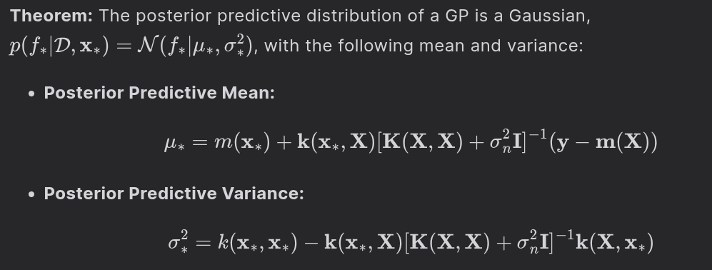
 , where
  . This is equivalent to the likelihood
  .
. , where
  are the training inputs and
  are the noisy training targets.
  at a new test point
  and the test output
  are jointly Gaussian –
 is the vector of prior means at the training points.
 is the
  covariance matrix where
  . The term
  is added to account for the independent observation noise.
 is the
  vector of covariances between the training points and the test point.
 is the prior variance at the test point.
 .
. .
.

 ): Controls how quickly the correlation between function values decays with distance. A small
  ): Controls the overall vertical variation of the function from its mean.
 are typically not set by hand. They are learned from the data by maximizing the marginal log-likelihood:
 , is a complexity penalty term that penalizes overly complex models.
 is the normalization constant. It ensures that the total area under the curve integrates to 1, as required for any valid PDF:
 and
and  is called the standard normal distribution, denoted
  can be transformed into a standard normal variable
 ): Approximately 68.27% of the area under the curve lies within one standard deviation of the mean.
 ): Approximately 95.45% of the area under the curve lies within two standard deviations of the mean.
 ): Approximately 99.73% of the area under the curve lies within three standard deviations of the mean.
 for scalars
 ![\mathbb{E}[Y] = \mathbb{E}[aX+b] = a\mathbb{E}[X]+b = a\mu + b](https://s0.wp.com/latex.php?latex=%5Cmathbb%7BE%7D%5BY%5D+%3D+%5Cmathbb%7BE%7D%5BaX%2Bb%5D+%3D+a%5Cmathbb%7BE%7D%5BX%5D%2Bb+%3D+a%5Cmu+%2B+b&bg=ffffff&fg=000&s=0&c=20201002)

 .
.  is said to have a multivariate Gaussian distribution if its Probability Density Function (PDF) is given by:
 .
.
 is the determinant of the covariance matrix, which geometrically represents the squared volume of the parallelepiped formed by the eigenvectors of


 are the eigenvectors of
  is a diagonal matrix of the corresponding non-negative eigenvalues
  .
. of
of  determine the spread along these axes. The length of the semi-axis along the direction
  .
. . Let’s partition this vector into two disjoint subsets,
  and
and  .
.

 are the mean vectors,
  are the covariance matrices of
  is the cross-covariance matrix.
 , if we have no information about the other?
 , if we observe the value of the other?

 .
.

 and is adjusted based on how surprising the observation
  ). The adjustment is scaled by the correlation term
  .
. minus a positive semi-definite term that represents the information gained from the observation.


 and mean
  of the resulting Gaussian are given by:

 is a scaling constant that does not depend on
  :
:
 and
and  .
. ![\mathbb{E}[\mathbf{y}] = \mathbb{E}[\mathbf{A}\mathbf{x} + \mathbf{b}] = \mathbf{A}\mathbb{E}[\mathbf{x}] + \mathbf{b} = \mathbf{A}\boldsymbol{\mu} + \mathbf{b}](https://s0.wp.com/latex.php?latex=%5Cmathbb%7BE%7D%5B%5Cmathbf%7By%7D%5D+%3D+%5Cmathbb%7BE%7D%5B%5Cmathbf%7BA%7D%5Cmathbf%7Bx%7D+%2B+%5Cmathbf%7Bb%7D%5D+%3D+%5Cmathbf%7BA%7D%5Cmathbb%7BE%7D%5B%5Cmathbf%7Bx%7D%5D+%2B+%5Cmathbf%7Bb%7D+%3D+%5Cmathbf%7BA%7D%5Cboldsymbol%7B%5Cmu%7D+%2B+%5Cmathbf%7Bb%7D&bg=ffffff&fg=000&s=0&c=20201002)


 is also a Gaussian. This is a special case of the linear transformation where
 ![\mathbf{x} = [X, Y]^\top](https://s0.wp.com/latex.php?latex=%5Cmathbf%7Bx%7D+%3D+%5BX%2C+Y%5D%5E%5Ctop&bg=ffffff&fg=000&s=0&c=20201002) ,
, ![\mathbf{A}=[1, 1]](https://s0.wp.com/latex.php?latex=%5Cmathbf%7BA%7D%3D%5B1%2C+1%5D&bg=ffffff&fg=000&s=0&c=20201002) , and
, and  . The resulting distribution is:
![p \in [0, 1]](https://s0.wp.com/latex.php?latex=p+%5Cin+%5B0%2C+1%5D&bg=ffffff&fg=000&s=0&c=20201002) , which represents the probability of success.
, which represents the probability of success.

![\mathbb{E}[X] = 1 \cdot p + 0 \cdot (1-p) = p](https://s0.wp.com/latex.php?latex=%5Cmathbb%7BE%7D%5BX%5D+%3D+1+%5Ccdot+p+%2B+0+%5Ccdot+%281-p%29+%3D+p&bg=ffffff&fg=000&s=0&c=20201002)
![\text{Var}(X) = \mathbb{E}[X^2] - (\mathbb{E}[X])^2 = (1^2 \cdot p + 0^2 \cdot (1-p)) - p^2 = p - p^2 = p(1-p)](https://s0.wp.com/latex.php?latex=%5Ctext%7BVar%7D%28X%29+%3D+%5Cmathbb%7BE%7D%5BX%5E2%5D+-+%28%5Cmathbb%7BE%7D%5BX%5D%29%5E2+%3D+%281%5E2+%5Ccdot+p+%2B+0%5E2+%5Ccdot+%281-p%29%29+-+p%5E2+%3D+p+-+p%5E2+%3D+p%281-p%29&bg=ffffff&fg=000&s=0&c=20201002)
 and the probability of success
  .
. failures is
  , due to independence.
 . Combining these gives the PMF:
 where
where  . Using the linearity of expectation and the property that the variance of a sum of independent variables is the sum of their variances:
![\mathbb{E}[K] = \mathbb{E}[\sum X_i] = \sum \mathbb{E}[X_i] = \sum p = np](https://s0.wp.com/latex.php?latex=%5Cmathbb%7BE%7D%5BK%5D+%3D+%5Cmathbb%7BE%7D%5B%5Csum+X_i%5D+%3D+%5Csum+%5Cmathbb%7BE%7D%5BX_i%5D+%3D+%5Csum+p+%3D+np&bg=ffffff&fg=000&s=0&c=20201002)
![\text{Var}(K) = \text{Var}[\sum X_i] = \sum \text{Var}[X_i] = \sum p(1-p) = np(1-p)](https://s0.wp.com/latex.php?latex=%5Ctext%7BVar%7D%28K%29+%3D+%5Ctext%7BVar%7D%5B%5Csum+X_i%5D+%3D+%5Csum+%5Ctext%7BVar%7D%5BX_i%5D+%3D+%5Csum+p%281-p%29+%3D+np%281-p%29&bg=ffffff&fg=000&s=0&c=20201002)
 , as the number of trials
  .
. one-second subintervals. Let the “success” be an event (e.g., a customer arriving) occurring in a subinterval. The probability
 is a normalization constant that ensures the probabilities sum to 1.
![\mathbb{E}[K] = \lambda](https://s0.wp.com/latex.php?latex=%5Cmathbb%7BE%7D%5BK%5D+%3D+%5Clambda&bg=ffffff&fg=000&s=0&c=20201002)


 , will always be positive, thus preventing the model from making impossible negative predictions. This logarithmic transformation is called a link function.
 .
.![\mathbf{x} = [0, \dots, 1, \dots, 0]^\top](https://s0.wp.com/latex.php?latex=%5Cmathbf%7Bx%7D+%3D+%5B0%2C+%5Cdots%2C+1%2C+%5Cdots%2C+0%5D%5E%5Ctop&bg=ffffff&fg=000&s=0&c=20201002) , where the 1 is in the
, where the 1 is in the 
 .
.![\mathbf{X} = [X_1, \dots, X_K]^\top](https://s0.wp.com/latex.php?latex=%5Cmathbf%7BX%7D+%3D+%5BX_1%2C+%5Cdots%2C+X_K%5D%5E%5Ctop&bg=ffffff&fg=000&s=0&c=20201002) follows a Multinomial distribution if each component
follows a Multinomial distribution if each component  represents the total count for the
  .
. outcomes of category 1,
  of category 2, …, up to
  of category
  ) is given by:
![\mathbb{E}[X_k] = np_k](https://s0.wp.com/latex.php?latex=%5Cmathbb%7BE%7D%5BX_k%5D+%3D+np_k&bg=ffffff&fg=000&s=0&c=20201002)
 (Each marginal is a Binomial)
 for
for  . The counts are negatively correlated because an increase in the count of one category must come at the expense of another.